MISO (Mixture of Isoforms) software documentation
- MISO (Mixture of Isoforms) software documentation
- What is MISO?
- How MISO works
- Mailing list
- Installation
- Overview
- Ways of running MISO and associated file formats
- Using MISO in parallel on multiple cores
- Using MISO on a cluster
- Alternative event annotations
- Running MISO
- Summarizing MISO output
- Detecting differentially expressed isoforms
- Compressing raw MISO output
- Example MISO pipeline
- Interpreting and filtering MISO output
- Visualizing and plotting MISO output
- Updates
- Frequently Asked Questions (FAQ)
- Advanced uses of MISO
- Acknowledgements
- Authors
- Installing Python-only MISO version
- References
What is MISO?
MISO (Mixture-of-Isoforms) is a probabilistic framework that quantitates the expression level of alternatively spliced genes from RNA-Seq data, and identifies differentially regulated isoforms or exons across samples. By modeling the generative process by which reads are produced from isoforms in RNA-Seq, the MISO model uses Bayesian inference to compute the probability that a read originated from a particular isoform.
The MISO framework is described in Katz et. al., Analysis and design of RNA sequencing experiments for identifying isoform regulation. Nature Methods (2010).
How MISO works
MISO treats the expression level of a set of isoforms as a random variable and estimates a distribution over the values of this variable. The estimation algorithm is based on sampling, and falls in the family of techniques known as Markov Chain Monte Carlo (“MCMC”). For details of the inference procedure, see Katz et. al. (2010).
Features
- Estimates of isoform expression (Ψ values, for “Percent Spliced In” or “Percent Spliced Isoform”) and differential isoform expression for single-end or paired-end RNA-Seq data
- Expression estimates at the alternative splicing event level (“exon-centric” analysis) or at the whole mRNA isoform-level (“isoform-centric” analysis)
- Confidence intervals for expression estimates and quantitative measures of differential expression (“Bayes factors”)
- Basic functionality for use on cluster / distributed computing system
Mailing list
Mailing list where users can ask technical questions is available at miso-users (http://mailman.mit.edu/mailman/listinfo/miso-users).
Installation
The primary version of MISO is called fastmiso – which is written in a combination of Python and the C programming language.
To install MISO, either download one of the stable releases (see Releases) or install the latest version from our GitHub repository. See below for detailed installation instructions.
Releases
MISO is available as a Python package, listed as misopy in pypi (Python Package Index).
Stable releases:
- MISO version 0.5.4 (misopy-0.5.4.tar.gz), July 20, 2017 release (Most recent)
- MISO version 0.5.3 (misopy-0.5.3.tar.gz), March 10, 2015 release
- MISO version 0.5.2 (misopy-0.5.2.tar.gz), March 11, 2014 release
- MISO version 0.5.1 (misopy-0.5.1.tar.gz), February 23, 2014 release
- MISO version 0.5.0 (misopy-0.5.0.tar.gz), February 21, 2014 release
- MISO version 0.4.9 (misopy-0.4.9.tar.gz), April 26, 2013 release
- MISO version 0.4.8 (misopy-0.4.8.tar.gz), April 14, 2013 release
- MISO version 0.4.7 (misopy-0.4.7.tar.gz), Christmas, 2013 release
- MISO version 0.4.6 (misopy-0.4.6.tar.gz), September 27, 2012 release
- MISO version 0.4.5 (misopy-0.4.5.tar.gz), September 4, 2012 release
- MISO version 0.4.4 (misopy-0.4.4.tar.gz), July 26, 2012 release
- MISO version 0.4.3 (misopy-0.4.3.tar.gz), June 1, 2012 release
- MISO version 0.4.2 (misopy-0.4.2.tar.gz), May 4, 2012 release
- MISO version 0.4.1 (misopy-0.4.1.tar.gz), February 1, 2012 release
- MISO version 0.4 (misopy-0.4.tar.gz), January 13, 2012 release
- MISO version 0.3 (misopy-0.3.tar.gz), January 8, 2012 release
- MISO version 0.2 (misopy-0.2.tar.gz), January 3, 2012 release
- MISO version 0.1 (misopy-0.1.tar.gz), Christmas, 2012 release
Latest version from GitHub
- Download latest MISO version from
fastmisoGitHub repository (.zip): https://github.com/yarden/MISO/zipball/fastmiso
Installation requirements
MISO requires a small number of Python modules and commonly used software like samtools for accessing SAM/BAM files. The requirements are:
Required Python modules:
- Python 2.6 or higher
- numpy and scipy. Note: MISO requires numpy version > 1.5!
- pysam, a Python library for working with SAM/BAM files through
samtools(Note: MISO requires pysam version 0.6 or higher)- matplotlib: Only required for use with
sashimi_plotfor plotting
Other required software:
We strongly recommend that you install MISO using a Python package manager (see Installing the fastmiso version of MISO) so that the required Python modules are automatically installed and managed for you.
Quickstart
To quickly start using MISO, follow these steps (each of which is described in detail in the rest of the manual):
Choose your GFF annotation set (see Alternative event annotations for our own annotations, available for human, mouse and fruit fly genomes.)
Index the annotation using
index_gff:index_gff --index SE.gff3 indexed_SE_events/
where SE.gff3 is a GFF file containing descriptions of isoforms/alternative splicing events to be quantitated (e.g. skipped exons).
- Run MISO:
Use
misoto get isoform expression estimates, optionally using a cluster to run jobs in parallel, e.g.:miso --run indexed_SE_events/ my_sample1.bam --output-dir my_output1/ --read-len 36 --use-cluster miso --run indexed_SE_events/ my_sample2.bam --output-dir my_output2/ --read-len 36 --use-clusterwhere
indexed_SE_eventsis a directory containing the indexed skipped exon events. Optionally, you can pack the MISO output to reduce the space and number of files taken up by the output:miso_pack --pack my_output1/ miso_pack --pack my_output2/
Summarize MISO inferences using
summarize_miso --summarize-samples:summarize_miso --summarize-samples my_output1/ summaries/ summarize_miso --summarize-samples my_output2/ summaries/
Make pairwise comparisons between samples to detect differentially expressed isoforms/events with
compare_miso --compare-samples:compare_miso --compare-samples my_output1/ my_output2/ comparison_output/
Parse and filter significant events with sufficient coverage.
For a full example of running MISO, see Example MISO pipeline. Also see the Frequently Asked Questions (FAQ) page.
- See MISO glossary for quick explanations of MISO terminology.
Installing the fastmiso version of MISO
The fastmiso version of MISO is written in a combination of C and Python. The underlying statistical inference engine is written in C and can be compiled on Mac OS X or Unix-like platforms using GCC or other standard compilers. The interface to this code is written in Python and is identical in its commands and input and output formats to the original Python-only version of MISO. (The Python-only version of MISO is now deprecated.)
There are two options for installing MISO, using either a stable release or installing the latest version from GitHub.
Installing using a stable release
It is highly recommended to install Python packages using a package manager such as the pip utility (see Python packaging tools tutorial for straightforward instructions on getting started.) Package managers will automatically download and install all necessary requirements for MISO and save headaches later on.
To install a stable release package of MISO using a Python package pip, simply type:
pip install misopy
This will install MISO globally, fetching and installing all of its required Python modules. To install MISO locally (without needing global installation access), it is best to use virtualenv in combination with pip. virtualenv will create a “virtual environment” where a package and all of its dependencies can be installed. The virtual environment can be loaded whenever needed and so it will not interfere with other (potentially conflicting) Python packages that are available on the system. If you’re a user working on a cluster system where you don’t have root privileges, all you need is pip and virtualenv to be available – the remaining installation steps can all be done locally without root access. To start, create a virtual environment (in this case called myenv) in a local directory to which you have write access (e.g. your home directory):
virtualenv myenv
This will create a directory myenv/ that contains a Python virtual environment. Next, install MISO in this local environment:
myenv/bin/pip install misopy
Finally, activate the environment in order to make all the executable MISO scripts available:
source myenv/bin/activate
This completes a local installation of the MISO Python package. To test the installation, load Python and import the misopy and pysplicing packages in the interpreter:
>> import misopy
>> import pysplicing
The miso main executable should be available on your path now:
$ miso
MISO (Mixture of Isoforms model)
Probabilistic analysis of RNA-Seq data for detecting differential isoforms
Use --help argument to view options.
If you get no errors, the installation completed successfully. Note that MISO also needs samtools to be installed and available on your path.
Installing the latest version from GitHub repository
To install the latest version from the GitHub repository, there are two options: (a) using git to get the latest source from our GitHub repository, or (b) by downloading a snapshot of the current repository, without going through git. If you have git installed and configured with your GitHub account, you can clone our repository as follows:
git clone git://github.com/yarden/MISO.git
This will create a directory called MISO, containing the repository. Alternatively, if you do not want to go through git, you can download a zip file containing the latest MISO GitHub release (following this link: https://github.com/yarden/MISO/zipball/fastmiso). This zip file has to be unzipped (e.g. using unzip fastmiso on Unix systems) and contains the latest release of the MISO repository.
Next, compile the code and install MISO using the Python package manager (such as as pip or `easy_install`_) as described above. We strongly recommend that you manage Python packages using a package manager rather than manually installing packages and modifying your PYTHONPATH, which is error prone and time consuming.
Testing the installation
To test if the required modules are available, use the
module_availability script as follows:
$ module_availability
Checking for availability of: numpy
Checking for availability of: scipy
...
All modules are available!
It is crucial that the samtools command is available from the
default path environment, or else MISO will not be able to parse
SAM/BAM files. On a Unix or a Mac OS X system, you should be able to
type samtools at the prompt and get access to the program without
specifying any path prefix.
To test that the MISO packages are properly installed, verify that the two modules misopy and pysplicing are available from your Python environment:
>> import misopy
>> import pysplicing
You should be able to import both of these packages without errors from the Python interpreter. The misopy package is the main MISO package, containing utilities for analyzing RNA-Seq data and plotting it (including sashimi_plot). The pysplicing package is an under-the-hood interface between Python and the statistical inference engine written in C.
Testing MISO
To test that MISO can be run properly, run the unit tests as shown below. These tests ensure that MISO can be run on a few genes/exons. The output of these tests can be ignored and the abbreviated version should be along the following lines:
$ python -m unittest discover misopy
Testing conversion of SAM to BAM...
...output omitted...
Computing Psi for 1 genes...
...
----------------------------------------------------------------------
Ran 3 tests in 68.000s
OK
If you see errors prior to this, the most likely cause is that some dependency
is not installed or not available in the path environment. For
example, if samtools is installed but missing from the path
(i.e. not accessible from the shell), that will cause errors in the
test run.
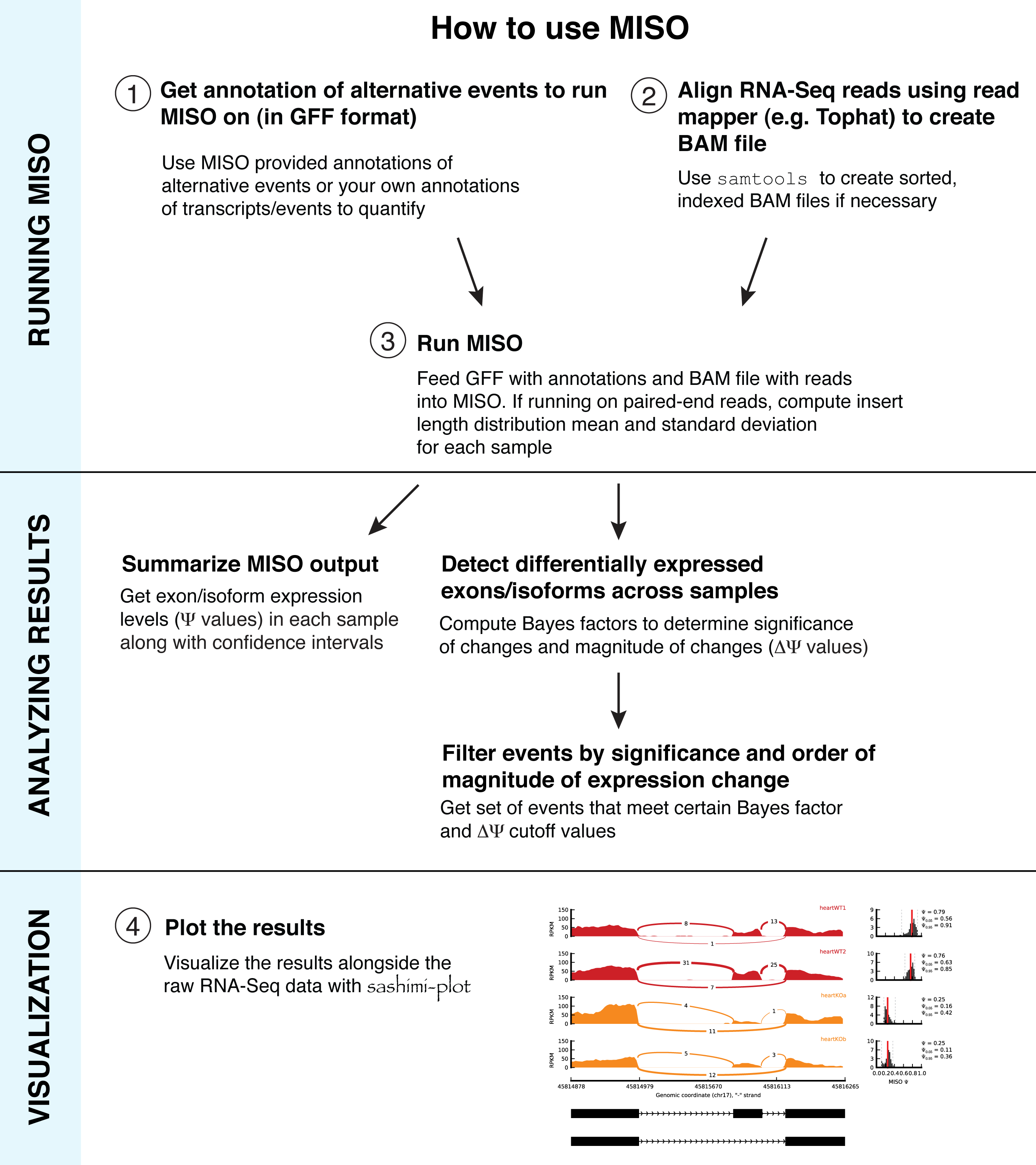
Overview
To run MISO, a set of annotations (typically specified in GFF format) of the isoforms of alternative events must be provided and RNA-Seq reads (typically specified in SAM format). The GFF annotation is indexed into an efficient representation using a script provided by MISO. The SAM reads must be sorted and indexed into the BAM format (binary version of SAM) before they can be used with MISO.
The sections that follow describe in detail the file formats used for the annotation and for the reads and the specific steps that are required to run MISO. An example of a MISO pipeline for computing isoform expression estimates and detecting differentially expressed isoforms is given in Example MISO pipeline.
The figure below shows an overview of how to run MISO.
Ways of running MISO and associated file formats
MISO can be run on either single or paired-end RNA-Seq data. Two general kinds of analyses are possible:
- Estimate expression level of exons (“exon-centric” analysis) or,
- Estimate expression level of whole transcripts (“isoform-centric” analysis)
Exon-centric analyses are recommended for looking at alternative splicing at the level of individual splicing events, e.g. the inclusion levels of a particular skipped exon, or the use of a particular alternative splice site. In isoform-centric analyses the expression level of whole isoforms for genes are estimated (i.e. the expression of each individual isoform of a gene is estimated). Both of these analysis modes have merits and disadvantages. Exon-centric analyses are typically easier to interpret and validate experimentally, but do not always capture the complexity of a set related splicing events within a gene. Isoform-centric analyses capture more of this complexity, but are limited by the typically short length of RNA-Seq reads, and inaccuracies or incompleteness in the annotation of the gene’s isoforms. Estimates of isoform-level expression are also harder to validate in the lab using traditional techniques such as RT-PCR.
To run MISO, an annotation of the alternative splicing events or isoforms must be provided and a set of reads. Single or paired-end reads can be provided in the Spliced Alignment/Map (SAM) format (in its binary form, BAM) and the annotation can be in the GFF (version 3) format. The GFF format can be used to specify either whole mRNA isoforms of genes (which is the common use of the format) or to specify single alternative splicing events, as described in Alternative event annotations.
Using MISO in parallel on multiple cores
When run locally and not on a cluster, MISO will use multiple cores on the machine on which it is running. The number of cores/processors to be used by MISO is set through the settings file (see Visualizing RNA-Seq reads along isoforms with MISO estimates).
Using MISO on a cluster
It is highly recommended to run MISO on a cluster when possible. Since each gene/exon can be treated as an independent inference problem, MISO is highly parallelizable, and the use of multiple computers can cut run times down by orders of magnitude.
MISO comes with basic functionality for running on a cluster, assuming that there’s a shared filesystem between all the nodes.
Alternative event annotations
Alternative event annotations are available for the major classes of alternative splicing and alternative RNA processing events in the human (hg18, hg19), mouse (mm9) and Drosophila melanogaster genomes. The event types covered are:
- Skipped exons (SE)
- Alternative 3’/5’ splice sites (A3SS, A5SS)
- Mutually exclusive exons (MXE)
- Tandem 3’ UTRs (TandemUTR)
- Retained introns (RI)
- Alternative first exons (AFE)
- Alternative last exons (ALE)
These annotations can be downloaded from the MISO annotations page.
For performing isoform-centric analyses, any gene models annotation can be used (e.g. from Ensembl, UCSC or RefSeq) as long as it is specified in the GFF3 format. As an example, we provide GFF3 annotations from Ensembl (which were converted from Ensembl’s GTF format to GFF3), available in Human/mouse gene models for isoform-centric analyses.
Expanded alternative cleavage and polyadenylation annotation for mouse
A recent paper from Bin Tian’s group, Analysis of alternative cleavage and polyadenylation by 3′ region extraction and deep sequencing, annotated alternative cleavage and polyadenylation events in mouse tissues using the 3′READS method. The annotated events (TandemUTR and ALE) are available in GFF format on the MISO annotations page, courtesy of the Tian group.
GFF-based alternative events format
Single alternative splicing events can be described in GFF format, using the convention described below. In the mouse and human genome event annotations in Alternative event annotations, alternative splicing events that produce two isoforms are described. For example, here is a skipped exon from the set of mouse skipped exons annotation (Version 1):
chr1  SE      gene    4772649 4775821 .       -       .       ID=chr1:4775654:4775821:-@chr1:4774032:4774186:-@chr1:4772649:4772814:-;Name=chr1:4775654:4775821:-@chr1:4774032:4774186:-@chr1:4772649:4772814:-
chr1  SE      mRNA    4772649 4775821 .       -       .       ID=chr1:4775654:4775821:-@chr1:4774032:4774186:-@chr1:4772649:4772814:-.A;Parent=chr1:4775654:4775821:-@chr1:4774032:4774186:-@chr1:4772649:4772814:-
chr1  SE      mRNA    4772649 4775821 .       -       .       ID=chr1:4775654:4775821:-@chr1:4774032:4774186:-@chr1:4772649:4772814:-.B;Parent=chr1:4775654:4775821:-@chr1:4774032:4774186:-@chr1:4772649:4772814:-
chr1  SE      exon    4775654 4775821 .       -       .       ID=chr1:4775654:4775821:-@chr1:4774032:4774186:-@chr1:4772649:4772814:-.A.up;Parent=chr1:4775654:4775821:-@chr1:4774032:4774186:-@chr1:4772649:4772814:-.A
chr1  SE      exon    4774032 4774186 .       -       .       ID=chr1:4775654:4775821:-@chr1:4774032:4774186:-@chr1:4772649:4772814:-.A.se;Parent=chr1:4775654:4775821:-@chr1:4774032:4774186:-@chr1:4772649:4772814:-.A
chr1  SE      exon    4772649 4772814 .       -       .       ID=chr1:4775654:4775821:-@chr1:4774032:4774186:-@chr1:4772649:4772814:-.A.dn;Parent=chr1:4775654:4775821:-@chr1:4774032:4774186:-@chr1:4772649:4772814:-.A
chr1  SE      exon    4775654 4775821 .       -       .       ID=chr1:4775654:4775821:-@chr1:4774032:4774186:-@chr1:4772649:4772814:-.B.up;Parent=chr1:4775654:4775821:-@chr1:4774032:4774186:-@chr1:4772649:4772814:-.B
chr1  SE      exon    4772649 4772814 .       -       .       ID=chr1:4775654:4775821:-@chr1:4774032:4774186:-@chr1:4772649:4772814:-.B.dn;Parent=chr1:4775654:4775821:-@chr1:4774032:4774186:-@chr1:4772649:4772814:-.B
The ID of the exon was chosen arbitrarily to be chr1:4775654:4775821:-@chr1:4774032:4774186:-@chr1:4772649:4772814:-. This name encodes the genomic coordinates of the upstream (5’) exon, the skipped exon, and
the downstream (3’) exon of this alternative splicing event, separated by @ symbols. The two isoforms that result (encoded as mRNA entries in the file) are: (1) the isoform made up of the upstream exon, the skipped exon and the
downstream exon (isoform where the exon is included), (2) the isoform made up of the upstream
exon followed by the downstream exon (isoform where the exon is skipped.) Note that we only use
the two flanking exons in this annotation, but one could modify the annotation to include arbitrarily many
flanking exons from the transcripts. We chose to name the two mRNA entries as the coordinates of the
exons that make up the mRNA followed by A for the first isoform, B for the second, though these
naming conventions are arbitrary and do not have to be used. Similarly, the ID of each exon is encoded
as its coordinate followed by up, se or dn to denote the upstream, skipped or downstream
exons, respectively.
Mapping of alternative events to genes
A mapping from alternative events to genes can be downloaded from the MISO annotations page.
Using GFF event annotations with paired-end reads
Note that in the above GFF annotations for events, only immediately flanking exons to an alternative event are considered. For example, for a skipped exon event, only the two exons that flank it are considered in the annotation. In the human/mouse genomes, this means that the two isoforms produced the event would be roughly ~400 nt and ~300 nt long. Modified annotations that use more of the exons present in the two isoforms might be more appropriate for use with long insert length paired-end libraries where the average insert is significantly longer than these isoform lengths. This in general will not affect isoform-centric analyses, where the entire mRNA transcript is used as the annotation to quantitate.
Human/mouse gene models for isoform-centric analyses
For isoform-centric analyses, annotations of gene models are needed, where whole mRNA isoforms are specified for each gene. Any annotation that is in GFF3 format can be used, e.g. annotations obtained from RefSeq, Ensembl, UCSC or other databases.
Annotations can be converted from UCSC table formats or from GTF format into GFF3 using the following procedure:
- Download your gene annotation (e.g. Ensembl genes, RefSeq) from UCSC Table Browser. For example, an Ensembl genes table
ensGene.txtcan be downloaded for themm9genome from UCSC goldenPath here (http://hgdownload.cse.ucsc.edu/goldenPath/mm9/database/ensGene.txt.gz).- To convert this gene table into GFF3, use of these two ways: (a) use the script ucsc_table2gff3.pl (from biotoolbox) to convert the table directly into GFF3, or (b) use the UCSC utility genePredToGtf to convert the table into GTF format (instructions for this are described in http://genomewiki.ucsc.edu/index.php/Genes_in_gtf_or_gff_format) and then convert the GTF file into GFF3 using gtf2gff3.pl.
For convenience, we provide GFF3 annotations based on UCSC Table Browser’s version of Ensembl genes for the following genomes:
- Mouse Ensembl genes from UCSC
- Annotation for mm9: mm9 ensGene GFF annotation
- Annotation for mm10: mm10 ensGene GFF annotation
- Human Ensembl genes from UCSC
- Annotation for hg18: hg18 ensGene GFF annotation
- Annotation for hg19: hg19 ensGene GFF annotation
It is critical to note that Ensembl and UCSC have distinct chromosome naming conventions (see warning note below). However, Ensembl tables obtained from the UCSC Table Browser will follow the UCSC chromosome naming conventions, not Ensembl’s, which is why the UCSC-downloaded Ensembl annotations in the GFFs provided above contain chr headers. Ensembl annotations obtained directly from Ensembl (e.g. via Ensembl BioMart) will of course follow the Ensembl chromosome naming conventions, and not UCSC’s.
Warning
The UCSC and Ensembl databases name their chromosomes differently. By convention, UCSC chromosomes start with
chrwhile Ensembl chromosome names do not. UCSC will call the fifth chromosomechr5and Ensembl will call it5. If your GFF annotation uses one convention, but your BAM reads are aligned to distinct headers, i.e. chromosome names following another convention, then none of your reads will map. For example, MISO will try to find all the regions onchr5if your GFF annotation follows the UCSC convention and fail, since all your BAM alignments could be to a header named5, or vice versa. In that case, lines such as these will appear in the MISO output:Cannot fetch reads in region: 5:1200-1500We strongly recommend that you check that your BAM files follow the same headers naming convention as your GFF. If you run into a mismatch between your annotation’s chromosome headers and your BAM file headers, please make sure that the headers that you map to in the read mapping stage to are the same as the headers used in the GFF annotation for MISO. For example, if you use TopHat/Bowtie to map reads and your genome index was made with UCSC-style
chrheaders but you want to use Ensembl annotations for quantitations, the solution is to:
- Download your genome’s sequence files (
*.fa, typically) from Ensembl,- Make a new Bowtie index from these files (using
bowtie-build), or the appropriate index for your read mapping program,- Remap your reads against this new index. The resulting mapped SAM/BAM files can be used with the unmodified Ensembl GFF annotations we provide here, where the headers in the GFF are guaranteed to match the headers in the SAM/BAM files (both using Ensembl header conventions.)
For convenience, we also provide GFF3 annotations of gene models from Ensembl (release 65), which were simply converted from Ensembl’s GTF to GFF3 format and are otherwise identical to the Ensembl annotation.
- Mouse Ensembl genes (16 M, .zip): Mus_musculus.NCBIM37.65.gff
- Human Ensembl genes (26 M, .zip): Homo_sapiens.GRCh37.65.gff
Running MISO
Invoking MISO from the command line
When installing the MISO package, the set of scripts that make up to inteface to MISO will automatically be placed as an executables in your path, so that you can refer to these without modifying your shell environment. For example, if you install MISO using setup.py install globally, then a MISO script like miso will become available on the path, and can be run as:
miso
The path of the Python version on the system used to install MISO will automatically be invoked when running these scripts.
If you installed MISO using setup.py --prefix=~/ in your home directory or some other path, these scripts will typically be placed in a designated executables directory in your home directory, e.g. ~/bin/.
Preparing the RNA-Seq reads
MISO can take as input RNA-Seq reads in the SAM format. SAM files are typically the output of read alignment programs, such as Bowtie or Tophat. The SAM format can represent both single and paired-end reads.
Files in SAM format must be converted to an indexed, sorted BAM file that contain headers. If you have an indexed, sorted BAM file you can move on to the next section.
The right BAM file can be created using samtools manually, or with the help of the wrapper
script sam_to_bam that calls samtools. For example, to convert my_sample.sam to an
indexed, sorted BAM file with headers specified in mm9_complete.fa.fai and output the result
to the directory my_sample/, use:
sam_to_bam --convert my_sample.sam my_sample/ --ref mm9_complete.fa.fai
The mm9_complete.fa.fai is a header file that contains the lengths of each chromosome
in the genome used to create the my_sample.sam file. The .fai files can be created from the
FASTA files of a genome using the faidx option of samtools (e.g. samtools faidx genome.fasta).
The sam_to_bam script will output a set of BAM files and their indices (my_sample.bam,
my_sample.sorted.bam, my_sample.sorted.bam.bai) to my_sample/.
Preparing the alternative isoforms annotation
To quantitate alternative splicing, an annotation file must be provided that describes the isoforms whose expression should be estimated from data.
To estimate the expression level of whole mRNA transcripts, a GFF format containing a set of annotated transcripts for each gene can be used. This is the same GFF that can be given as input to Tophat in order to incorporate known genomic junctions, for example. These GFF files can be readily produced for any annotated genome (see Human/mouse gene models for isoform-centric analyses for Ensembl-based annotations of this form for human/mouse genomes.)
For exon-centric analyses, a GFF file can be used as well, except such a file will contain only the subsets of the isoforms produced by a particular splicing event – rather than whole transcripts – as described in GFF-based alternative events format. The GFF file chosen has to be indexed for efficient representation. A set of indexed, ready-to-use events is available for the mouse and human genomes.
To create an index for the GFF annotations, the index_gff script can be used as follows:
index_gff --index SE.mm9.gff indexed/
This will index the GFF file SE.mm9.gff and output the result to the indexed/ directory.
This indexed directory is then used as input to MISO.
Configuring MISO
The default configuration file for MISO is available in settings/miso_settings.txt.
Skip to the next section if you’d like to use the default configuration file.
The default file is:
[data]
filter_results = True
min_event_reads = 20
strand = fr-unstranded

[cluster]
cluster_command = qsub

[sampler]
burn_in = 500
lag = 10
num_iters = 5000
num_processors = 4
The [data] section contains parameters related to the way reads should be handled. These are:
filter_results: Specifies whether or not events should be filtered for coverage (TrueorFalse)min_event_reads: What the minimum number of reads that a region must have for it to be quantitated. The minimum number of reads is computed over the longest genomic region of the gene or alternatively spliced event.strand(optional): What the strand convention of the input BAM files is. Can be set to eitherfr-unstranded,fr-firststrand, orfr-secondstrand. Set tofr-unstrandedby default. See Note on strand-specificity in RNA-Seq libraries for an explanation of these strand conventions.
The [cluster] section specifies parameters related to running MISO on a cluster of computers.
These are:
cluster_command: the name of the program used to submit jobs to the cluster (e.g.qsub,bsub, etc.) MISO will use this command to launch jobs on the cluster system.long_queue_name(optional): the name of the “long queue” (jobs that take longer to finish) of the cluster queueing system.short_queue_name(optional): the name of the “short queue” (jobs that generally finish quicker and might get priority) of the cluster queueing system. The name of this queue is oftenshortorquickdepending on the way the cluster is configured.
Both long_queue_name and short_queue_name can be omitted from the configuration file, in which
case jobs will be submitted to the cluster without specifying any queue. All parameters set in the
[clusters] section are only relevant when MISO is used on a cluster.
The [sampler] section specifies internal parameters related to MISO’s sampling algorithm. Most users
will not want to tweak these. The parameters are as follows:
burn_in: the number of initial sampling iterations to be discarded before computing estimates.lag: the number of sampling iterations to skip when computing estimates. A lag of 10 would mean every 10th iteration is used.num_iters: the total number of sampling iterations to be computed per gene/event.num_processors(optional): Number of processors to use when running locally using multiple cores. Set to 4 by default. Not used when running on a cluster.
The default settings of the sampling-related parameters in [sampler] was deliberately chosen to be conservative.
Computing expression estimates (“Psi” / Ψ values)
To run MISO to estimate the expression level of a set of annotated isoforms or events in GFF format,
the miso script is used with the --run option.
This produces distributions over “Psi” values (Ψ), which stand for
“Percent Spliced In”. See Katz et. al. (2010) for a description of
these values and how they are computed.
Using single-end reads
The --run takes the following arguments:
--run
                      Compute Psi values for given GFF annotation.
                      Expects two arguments: an indexed GFF
                      directory with genes to process, and a sorted, indexed
                      BAM file (with headers) to run on.
For example, to run on a single-end sample:
miso --run mm9/pickled/SE data/my_sample.sorted.bam --output-dir my_sample_output/ --read-len 35
This will compute expression values for the isoforms described in the indexed GFF directory mm9/pickled/SE, based on the reads in data/my_sample.sorted.bam (a sorted, indexed BAM file) an output the results to the my_sample_output/ directory. Note that the mm9/pickled/SE directory in this case must be generated by the user, by running index_gff.
The --read-len option is necessary and specifies the length of the reads in the data (in this case, 35 nt.) The directory mm9/pickled/SE, which is available in the mouse splicing event annotations, specifies an indexed version of all the skipped exon (SE) events.
Note that that the headers for the indexed/sorted BAM file (the files with the .bam.bai extension)
must be in the same directory as the read BAM file. In the above example, it means they must be in the
data/ directory.
If reads were aligned to a set of splice junctions with an overhang constraint — i.e., a requirement
that N or more bases from each side of the junction must be covered by the read — then this can be
specified using the --overhang-len option:
--overhang-len
                      Length of overhang constraints imposed on junctions.
Using paired-end reads
To compute expression levels using paired-end reads, use the --paired-end option:
--paired-end
                      Run in paired-end mode. Takes mean and standard
                      deviation of insert length distribution.
The insert length distribution gives the range of sizes of fragments sequenced in the
paired-end RNA-Seq run. This is used to assign reads to isoforms probabilistically.
The insert length distribution can be computed by aligning read pairs to long, constitutive
exons (like 3’ UTRs) and measuring the distance between the read mates. The mean and standard
deviation of this distribution would then be given as arguments to --paired-end.
For example, to run on a paired-end sample where the mean insert length is 250 and the standard
deviation is 15, we would use: --paired-end 250 15 when calling miso
(in addition to the --run option).
The --overhang-len option is not supported for paired-end reads.
Computing the insert length distribution and its statistics
We provide a set of utilities for computing and plotting the insert length distribution in paired-end RNA-Seq samples. The insert length distribution of a sample is computed by aligning the read pairs to long constitutive exons and then measuring the insert length of each pair. The set of insert lengths obtained this way form a distribution, and summary statistics of this distribution – like its mean and standard deviation – are used by MISO to assign read pairs to isoforms.
The utilities in exon_utils and pe_utils can be used to first get a set of long constitituve exons to map read pairs to, and second compute the insert length distribution and its statistics.
Getting a set of long constitutive exons: When computing the insert length distribution, it’s important to use exons that are significantly larger than the insert length that was selected for in preparing the RNA-Seq library. If the insert length selected for in preparing the RNA-Seq library was roughly 250-300 nt, we can use constitutive exons that are at least 1000 bases long, for example, so that both read pairs will map within the exon and not outside of it. The requirement that the exons be constitutive is to avoid errors in the insert length measurements that are caused by alternative splicing of the exon (which could alter the insert length.)
We first get all constitutive exons from a gene models GFF, like the Ensembl annotation of mouse genes (available here, Mus_musculus.NCBIM37.65.gff), we use exon_utils:
exon_utils --get-const-exons Mus_musculus.NCBIM37.65.gff --min-exon-size 1000 --output-dir exons/
This will output a GFF file (named Mus_musculus.NCBIM37.65.min_1000.const_exons.gff) into the exons directory containing only constitutive exons that are at least 1000 bases long. This file can be used to compute the insert length distribution of all mouse RNA-Seq datasets. Exons here are defined as constitutive only if they occur in all annotated transcripts of a gene.
Computing the insert length distribution given a constitutive exons file: Now that we have a file containing the long constitutive exons, we can compute the insert length for any BAM file using the pe_utils utilities. The option --compute-insert-len takes a BAM file with the RNA-Seq sample and a GFF file containing the long constitutive exons. The insert length is defined simply as the distance between the start coordinate of the first mate in the read pair and the end coordinate of the second mate in the read pair.
To compute the insert length for sample.bam using the constitutive exons file we made above, run:
pe_utils --compute-insert-len sample.bam Mus_musculus.NCBIM37.65.min_1000.const_exons.gff --output-dir insert-dist/
This will efficiently map the BAM reads to the exons in the GFF file using bedtools, and use the result to compute the insert lengths. The command requires the latest version of bedtools to be installed, where the tagBam utility was added the ability to output the interval that each read maps to in its BAM output file. The reads that aligned to these exons will be kept in a directory called bam2gff_Mus_musculus.NCBIM37.65.min_1000.const_exons.gff/ in the insert-dist directory.
This will generate an insert length distribution file (ending in .insert_len) that is tab-delimited with two columns, the first specifying the exon that the read pairs were aligned to, and the second specifying a comma-separated list of insert lengths obtained from aligning the read pairs to that exon. The number of entries in the file corresponds to the number of exons from the original GFF that were used in computing the insert length distribution.
The first line (header) of the the insert length file gives the mean, standard deviation and dispersion values for the distribution, for example:
#mean=129.0,sdev=12.1,dispersion=1.1,num_pairs=862148
This indicates that the mean of the insert length distribution was 129, the standard deviation was 12.1, dispersion was 1.1, and the number of read pairs used to estimate the distribution and compute these values was 862,148.
The dispersion constant d is defined as the standard deviation σ of the insert length distribution divided by the square root of its mean μ:
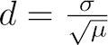
Dispersion constant d of an insert length distribution
Intuitively, the dispersion constant d corresponds to how variable the insert length distribution is about its mean. The lower the d value is, the tighter/more precise the insert length distribution is in the RNA-Seq sample. The dispersion constant and an interpretation of its values is discussed in the MISO paper (see Analysis and design of RNA sequencing experiments for identifying isoform regulation).
The insert length distribution can be plotted using the .insert_len file using sashimi_plot.
To compute the insert length by simple pairing of read mates by their ID (assuming that mates belonging to a pair have the same read ID in the BAM), explicitly ignoring the relevant BAM fields specifying whether or not the reads are properly paired, use the --no-bam-filter option.
Note
The option
--compute-insert-lencan take a comma-separated list of BAM filenames in case you want to compute the insert length for multiple samples in one command. The--compute-insert-lenoption ofpe_utilsby default uses only exons from the GFF file that are 500 bases or longer. This can be tweaked by passingpe_utilsthe optional--min-exon-size Nargument, which will only use exons of sizeNor longer. In our example, we used a constitutive exons GFF file that contained only exons that are 100 bp or longer, so the default settings will consider all exons in that file.
Prefiltering MISO events
To increase efficiency, a prefiltering option was added in release 0.4.7. When --prefilter is given to miso, MISO will calculate the number of reads in the input BAM mapping to each event in the input GFF. Events that do not meet the read coverage thresholds (as set in the configuration file) will be removed from the run. This feature requires the Bedtools utility tagBam to be installed and available on path. The call to tagBam introduces a startup cost per BAM file, but could in many cases save computation time, since events low coverage events will not processed or distributed as jobs to nodes when running on the cluster. From miso --help:
--prefilter           Prefilter events based on coverage. If given as
                      argument, run will begin by mapping BAM reads to event
                      regions (using bedtools), and omit events that do not
                      meet coverage criteria from the run. By default,
                      turned off. Note that events that do not meet the
                      coverage criteria will not be processed regardless,
                      but --prefilter simply does this filtering step at the
                      start of the run, potentially saving computation time
                      so that low coverage events will not be processed or
                      distributed to jobs if MISO is run on a cluster. This
                      options requires bedtools to be installed and
                      available on path.
Distributing MISO jobs to a cluster
Running MISO on a cluster is highly recommended. Since each gene or alternative splicing event can be treated independently, the computation of expression levels is easily parallelized on a cluster. This can reduce run times significantly, from days to hours on typical data sets. To run MISO on the cluster, the following options can be used:
--use-cluster: causes jobs to be sent to a cluster--chunk-jobs N(optional): placesNmany genes or events into each job. For example, if running MISO on a set of skipped exons,--chunk-jobs 200will place roughly 200 exons whose expression is to be estimated into each job. If each job was sent to a separate node, it would mean every node in parallel will sequentially compute the expression level of 200 exons. The value of--chunk-jobsdepends on both cluster size/availability and on the number of exons whose expression is to be estimated. On very large clusters where nodes are generally available, a relatively small setting of--chunk-jobsis likely to be more efficient.--no-wait(optional): by default, the main process that submits the jobs to the cluster will wait for them to finish. If--no-waitis passed, the main process will not wait, and simply quit after submitting the jobs.
MISO will use the cluster submission and queue settings described in the settings file to submit jobs (see Visualizing RNA-Seq reads along isoforms with MISO estimates). An example of a MISO pipeline for computing isoform expression estimates and detecting differentially expressed isoforms is given in Example MISO pipeline.
To use MISO on Sun Grid Engine, the following options to miso can be used:
--SGEarray: Run jobs on Sun Grid Engine. To be used in conjunction with--use-cluster.--job-name: Name the job submitted to Sun Grid Engine system.
Thanks to Michael Lovci for this feature.
Raw MISO output format
When running MISO, through miso --run, the raw output will be a set of posterior distributions over Ψ values. Each exon or gene, depending on whether the analysis is exon or isoform-centric, will have its own file containing posterior samples from the distribution over Ψ.
Most users will never need to access these raw distributions and can simply summarize this raw output as described in Summarizing MISO output, or perform a comparison between a set of samples as described in Detecting differentially expressed isoforms.
Each gene or exon will have a corresponding distribution file (ending in .miso), split into subdirectories by chromosome. The resulting directory structure might be:
my_sample_output/
  chr1/
  chr2/
  ...
  chrX/
The distribution file for an event, e.g. chr1/my_exon.miso, will contain tab-separated columns that specify the sampled Ψ values and the log score under the MISO model for each sample, e.g.:
#isoforms=['TandemUTRCore_TandemUTRExt','TandemUTRCore']      exon_lens=('TandemUTRCore',1986),('TandemUTRExt',1021)  iters=5000      burn_in=500     lag=10  percent_accept=92.90    proposal_type=drift
sampled_psi   log_score
0.0691,0.9309 -989.1296
0.0692,0.9308 -1002.1173
0.0595,0.9405 -994.5029
0.0587,0.9413 -988.9871
0.0539,0.9461 -980.4465
0.0571,0.9429 -986.1921
0.0482,0.9518 -980.2666
0.0392,0.9608 -999.4088
The header line (beginning with #) gives information about the gene/event in the file, like the names of the isoforms in the annotation and the length of the exons, as well as values of internal MISO parameters (like burn-in or lag, described in Visualizing RNA-Seq reads along isoforms with MISO estimates).
The first column (sampled_psi) lists the Ψ value sampled and the second column (log_score) gives the log score of that sample under the MISO model. The Ψ value is comma-separated and will have as many entries as there are isoforms. In the above file, there are two isoforms, and so two entries in the Ψ column that sum to 1.
After raw MISO output is summarized and all pairwise comparisons between samples have been made, the raw output can be compressed (see Compressing raw MISO output.)
Summarizing MISO output
To summarize MISO output and obtain confidence intervals (CIs) for Ψ values, the summarize_miso --summarize-samples option can be used:
--summarize-samples
                       Compute summary statistics of the given set of
                       samples. Expects a directory with MISO output and
                       a directory to output summary file to.
For example, to summarize the MISO output in my_sample_output/, run:
summarize_miso --summarize-samples my_sample_output/ summary_output/
This will create a subdirectory summary_output/summary/ with a file my_sample_output.miso_summary that summarizes all the events in the sample in my_sample_output/.
Summary file output format
The summary file is a tab-separated format containing the following columns:
event_name: name of the event or gene from the input annotation,miso_posterior_mean: an estimate of Ψ (derived by taking the mean of the posterior distribution over Ψ),ci_low: the low bound of the 95% confidence interval on the Ψ estimate,ci_high: the high bound of the 95% confidence interval on the Ψ estimate.isoforms: the names of the isoforms that make up the event/gene quantitated (from the input annotations)counts: raw read counts that support each isoform. Lists the number of reads that support each combination of isoforms. Each read type is represented as a comma-separated list (enclosed in parentheses) with number of entries equal to the number of isoforms quantitated, and a 1 or 0 in each entry depending on whether the read was consistent or inconsistent with the isoform. For example, for an alternative event with two isoforms, the entry might be:(1,0):28,(0,1):50,(1,1):12, where0and1correspond to the first and second isoforms. This indicates that 28 reads support isoform 1 but not 2, while 50 reads support the second but not the first, and 12 reads support both isoforms. The field(0,0):N, if outputted, indicates the number of readsNthat mapped to the region but were thrown out (e.g. because they are not consistent with the isoforms in the annotation, violate overhang constraints, or other related reasons.)assigned_counts: inferred assignment of reads to isoforms. Lists each isoform (0-based) and the number of reads assigned to it. For example, for an alternative event with two isoforms, the entry might be:0:330,1:34, indicating that 330 reads were assigned to the first isoform (isoform 0) and 34 reads were assigned to the second isoform (isoform 1).
Starting with release misopy-0.4.1, three additional columns are outputted with information about the gene/event (which are read from the input GFF annotation):
chrom: chromosome namestrand: strand of gene/eventmRNA_starts: comma-separated list of start genomic coordinates formRNAentries in gene/eventmRNA_ends: comma-separated list of end genomic coordinates formRNAenries in gene/event
When one of those fields is not available (e.g. strand), NA is outputted in its place.
Note that miso_posterior_mean is an estimate of Ψ and [ci_low, ci_high] are the 95% confidence limits of that estimate.
Detecting differentially expressed isoforms
Once MISO output has been computed for two samples or more, pairwise comparison of differential isoform expression can be computed. To test if an isoform or exon is differentially expressed between between samples, the Bayes factor is computed for the exon, which represents the weight of the evidence in the data in favor of differential expression versus not. For example, a Bayes factor of 2 would mean that the isoform/exon is two times more likely to be differentially expressed than not. The computation of Bayes factors is described in detail in Katz et. al. (2010).
To compute Bayes factors, the compare_miso --compare-samples option can be used. For example:
compare_miso --compare-samples control/ knockdown/ comparisons/
This would compare the MISO output in control/ to knowndown/, and output the result
to the directory comparisons/control_vs_knockdown. Note that
“vs” is used to denote sample comparisons. The output format of
this comparison is described below.
Output of samples comparison
The main output of --compare-samples will be in:
bayes-factors/: contains the file summarizing the output with the Bayes factors (ending in.miso_bf)
Bayes factors file output format
The Bayes factors file (ending in .miso_bf) will be stored in the bayes-factors/ directory generated
by the --compare-samples option. The Bayes factor file is a tab-separated format containing the following columns:
event_name: name of the event from the input annotation file,sample1_posterior_mean: Estimate of Ψ (mean of posterior distribution) for sample 1,sample1_ci_low: Low bound of 95% confidence interval for sample 1 Ψ estimate,sample1_ci_high: High bound of the 95% confidence interval for sample 1 Ψ estimate,sample2_posterior_mean: Estimate of Ψ (mean of posterior distribution) for sample 2,sample2_ci_low: Low bound of 95% confidence interval for sample 2 Ψ estimate,sample2_ci_high: High bound of 95% confidence interval for sample 2 Ψ estimate,diff: The difference (Δ Ψ) between sample 1 and sample 2 Ψ estimates, i.e.sample1_posterior_mean - sample2_posterior_meanbayes_factor: Bayes factor for the comparison, corresponding to the odds of differential expression ,where the change in Ψ is non-zero) over no differential expression (where the change is zero),isoforms: the names of the transcripts or events that were quantitated (based on the input annotation),sample1_counts: raw counts for sample 1 for each read type (same format as thecountsfield described in Summary file output format),sample1_assigned_counts: inferred assignment of reads to isoforms in sample 1 (same format as theassigned_countsfield described in Summary file output format),sample2_counts: raw counts for sample 2 for each read type,sample2_assigned_counts: inferred assignment of reads to isoforms in sample 2
If MISO is run on an annotation that specifies more than two isoforms per event/gene, then the fields for the Ψ estimates become comma-separated and give the estimates for each isoform. For example, in the case of three isoforms, sample1_ci_low would be a comma-separated list of the lower bounds of the first, second and third isoform, and sample1_ci_high would be a comma-separated list of the upper bounds of the first, second and third isoform, and similarly for the fields involving the other sample.
Starting with release misopy-0.4.1, three additional columns are outputted with information about the gene/event (which are read from the input GFF annotation):
chrom: chromosome namestrand: strand of gene/eventmRNA_starts: comma-separated list of start genomic coordinates formRNAentries in gene/eventmRNA_ends: comma-separated list of end genomic coordinates formRNAenries in gene/event
When one of those fields is not available (e.g. strand), NA is outputted in its place.
Compressing raw MISO output
Packing MISO output
Starting from version 0.5.0, the miso_pack utility is available for packing raw MISO output. The packing utility converts the raw MISO output directories that contain *.miso files and converts them into a portable SQLite database (one database file per chromosome.) This reduces the number of files substantially, which otherwise could burden the filesystem. The packing operation uses the built-in SQL library of Python (sqlite3) and does not require installation of any external SQL databases.
All downstream analyses analyses (like sample summary and comparisons, as described in Summarizing MISO output and Detecting differentially expressed isoforms) work with the packed format, and so there is never a need to ‘unpack’ MISO output once miso_pack was run. To pack a directory miso_output/ that contains output from MISO, run:
miso_pack --pack miso_output/
The miso_pack utility will traverse the entire directory structure of miso_output and pack any directories that contain raw MISO output.
Note: The SQLite databases made by miso_pack can be read independently of Python and queries as ordinary SQLite databases. However, end-users should never need to deal with these files directly.
Long-term archival and compression of MISO output
Once all the samples have been summarized and all pairwise comparisons between samples have been made (as described in Summarizing MISO output and Detecting differentially expressed isoforms), space can be saved by archiving the MISO output for long-term storage.
To compress directories containing raw MISO output files, a utility called miso_zip can be used. For example, to compress the directory miso_output/ into and name the result mydata.misozip, use:
miso_zip --compress mydata.misozip miso_output/
(Note that compressed MISO files must end in .misozip.) If miso_output is not already packed, miso_zip will first pack it, and then compress the result using standard zip comrpession to save space. miso_zip will take as argument any directory containing *.miso files (either directory within it or within its subdirectories)
This compression reduces the number of files dramatically, since each sample gets one SQLite database per chromosome. The resulting directory structure is then compressed further using standard zip compression into a single zip file (in this case named mydata.zip).
The compressed .misozip files can be uncompressed using miso_zip as follows:
miso_zip --uncompress mydata.misozip uncompressed/
This will uncompress mydata.misozip and output its contents into the directory uncompressed/.
Note: miso_zip will not delete the directory being compressed. The directory can be deleted manually after compression is done.
Example MISO pipeline
Below is an example of a MISO pipeline, where Ψ values for a set of alternative events are computed (with confidence intervals) for a pair of samples called “control” and “knockdown”. A samples comparison is performed to detect differentially expressed isoforms between the samples.
## Run MISO on a pair of paired-end sample (with insert length distribution with mean 250,
## standard deviation 15) using the mouse genome skipped exon annotations using the
## the cluster

# Compute Psi values for control sample
miso --run mm9/pickled/SE data/control.bam --output-dir SE/control/ --read-len 35 --paired-end 250 15 --use-cluster

# Compute Psi values for knockdown sample
miso --run mm9/pickled/SE data/knockdown.bam --output-dir SE/knockdown/ --read-len 35 --paired-end 250 15 --use-cluster


## Summarize the output (only run this once --run finished!)
## This will create a "summary" directory in SE/control/ and in SE/knockdown/
summarize_miso --summarize-samples SE/control/ SE/control/
summarize_miso --summarize-samples SE/knockdown/ SE/knockdown/

## Detect differentially expressed isoforms between "control" and "knockdown"
## This will compute Bayes factors and delta Psi values between the samples
## and place the results in the directory SE/comparisons/control_vs_knockdown
compare_miso --compare-samples SE/control/ SE/knockdown/ SE/comparisons/
Interpreting and filtering MISO output
Once MISO runs are completed and pairwise comparisons between your samples have been made to compute Bayes factors (using --compare-samples), the resulting files can be interpreted to detect differential events. For each pairwise comparison, we will have a .miso_bf file which contains the Ψ values of each event in both samples along with confidence intervals (assuming the event is detectable in both), the Δ Ψ values, the Bayes factor, and other useful information about the read counts used to compute these values.
MISO comes with several utilities (such as filter_events, described in Filtering differentially expressed events) for helping with the interpretation and analysis of these output files. This section serves as a brief guide the MISO output files, the utilities for analyzing them, and to various caveats in interpreting the output.
Using the read class counts
A first-pass filter for detecting differentially changing events can apply a Bayes factor cutoff along with a Δ Ψ cutoff, using the bayes_factor and diff fields of the samples comparison output file. Section Filtering differentially expressed events describes a utility that will apply these filters for exon-centric analyses.
It is critical to note that the default MISO settings were intentionally set to be highly inclusive, and therefore do not impose any stringent coverage criteria on the events for which Ψ values and Bayes factors are computed.
Note
By default, MISO requires only 20 reads to be present in the locus/event of interest. For many events, only a tiny fraction of these reads might be in informative regions – like junctions or regions unique to one of the isoforms – and so the expression levels of these events might not be reliably estimated. It is important to use the information provided by MISO about the raw number of read counts used in estimating the expression levels of each event/gene.
In addition to Ψ values, confidence intervals and Bayes factors, the output files of MISO (such as summary files or sample comparison files) also contain the number of read counts informative about each isoform.
The relevant read counts are given in the counts field of the .miso, .summary, .miso_bf files – its format is described in detail in Summary file output format). For the two-isoform case in exon-centric analyses, the counts field general format is:
(1,0):X,(0,1):Y,(1,1):Z,(0,0):L
where X, Y, Z, L are integer counts corresponding to the number of reads in each of these categories. Class (1,0) are reads consistent with the first isoform in the annotation but not the second, class (0,1) are reads consistent with the second but not the first, class (1,1) are consistent with both isoforms, and reads in (0,0) are consistent with neither. These are illustrated graphically in the figure below for alternatively skipped exon event:
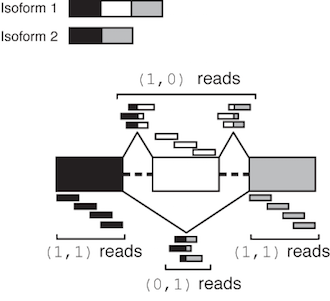
Illustration of MISO output read class counts for a skipped exon
The class (0,0) denotes reads that were incompatible with either isoform, either because they didn’t match these isoforms or were otherwise unusable (e.g. they were part of a read-pair where one end was unmappable, in the case of paired-end reads.) Reads in this class are not used by MISO – they are only reported to indicate that they were discarded.
Warning
Events that meet the very minimal default coverage criteria do not necessarily have sufficient read support to be considered alternatively spliced in your RNA-Seq samples.
In practice, events that might not be alternatively spliced in the samples of interest meet the default minimal read coverage criteria, although their read class counts imply that they are not reliable estimates. Such a case might be an alternative exon in the input annotation to MISO that has, for example, 19 reads in the exon upstream of the skipped exon, and 1 read in the exon downstream of the skipped exon. This event would have a counts signature of: (1,1):20,(1,0):0,(0,1):0. The (1,0) and (0,1) reads, which are most informative about the relative inclusion levels of the exon, are both 0, so unless these are non-zero in other samples in the dataset, the estimate of the inclusion levels of this exon will not be reliable.
For this reason, coverage filters must be imposed by the user when post-processing MISO output. An example of such a filter is given below for exon-centric analyses.
Tip
A commonly-used coverage filter in exon-centric (two-isoform) analyses requires the following minimal counts criteria to be met:
X + Y >= N, Y >= 1in at least one of the RNA-Seq samples processed by MISO, where
X, Yare the number of reads in the(1,0)and(0,1)read classes, respectively, andNis an arbitrary but sizeable number (e.g. 10 or 20). This filter requires that the sum of inclusion and exclusion-supporting reads be greater than or equal toN, and that the read class supporting exclusion is non-zero in at least one of the samples. This guarantees that at least some of the reads are informative about the inclusive or exclusive isoform. Note that this filter does not guarantee that there will be junction evidence for the inclusion isoform, but does guarantee that there will be a junction evidence for skipping of the exon.
To increase power to detect differential events, coverage filters should be applied in aggregate across all RNA-Seq samples that were processed by MISO. To detect switch-like exons that are fully included in one sample and fully excluded in another, we should require the number of exon exclusion supporting reads be non-zero in at least one of the samples – or summed across samples – rather than in every sample. This filter can be easily applied by parsing the counts field in the samples comparison (.miso_bf) file produced by MISO for each pairwise comparison.
For isoform-centric analyses where the number of read classes is considerably larger, MISO will output the counts in the same format. For a gene with 3 isoforms, we can have the read classes (1,0,0),(0,1,0),(0,0,1),...,(1,1,1) and other filters can be applied, depending on the goal of the analysis, to select genes that have sufficient coverage to be reliably estimated.
Using the confidence intervals
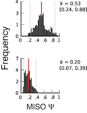
Important information is contained in the confidence intervals outputted by MISO for each estimate of Ψ. The width of the interval corresponds to our confidence in the estimate of the Ψ value, and so the larger the confidence width is, the less reliable the estimate. As expected, the width of the confidence interval will depend on the number of informative reads, such as reads crossing junctions or reads in regions that uniquely identify the isoform.
The figure on the right shows two posterior distributions over Ψ for the same alternative splicing event in two samples, where the exon had low coverage (i.e. small number of reads) in both. The posterior distribution is plotted as a black histogram, whose mean is indicated by the red vertical line and 95% confidence intervals shown by dotted grey vertical lines. The actual Ψ values and the confidence interval bounds are given to the right of the distribution. In the top distribution, the confidence interval width is .64 (since .88 - .24 = .64) which is extremely wide. The distribution’s probable range spans from 20 to nearly 90%, far too broad to be useful. In the bottom distribution, the confidence intervals are narrower, though still considerable. Because of the large amount of uncertainty in the top distribution, we cannot confidently conclude that the true Ψ value is likely to be different between the two. Although the difference of means between the distributions is large (.53 - .2 = .33), the confidence intervals overlap considerably as a result of the uncertainty in the top distribution. In practice, requiring no overlap at all between the confidence intervals of two samples is too restrictive, but the width of each estimate’s confidence interval and the relationship between the intervals should be kept in mind when interpreting the results.
Filtering differentially expressed events
Given a MISO Bayes factor comparison file for two-isoform events, events can be filtered based on their coverage or magnitude of change. The filter_events script allows filtering of events, based on the following criteria:
--num-total N: Number of total reads aligning to any isoform (or to both isoforms) has to be greater than or equal to N.--num-inc N: Number of inclusion reads (i.e. reads supporting the first isoform) has to be greater than or equal to N.--num-exc N: Number of exclusion reads (i.e. reads supporting the second isoform) has to be greater than or equal to N.--num-sum-inc-exc N: The sum of inclusion and exclusion reads has to be greater than or equal to N.--delta-psi P: The absolute Δ Ψ value must be greater than or equal to P (where P is in [0, 1]).--bayes-factor N: The Bayes factor must be greater than or equal to N.--apply-both: By default, the above filters on read coverage of the isoforms are required to be true in only one of the samples. To consider only events where the filters apply in both samples, use this option.
For example, to filter the file control.miso_bf to contain only events with: (a) at least 1 inclusion read, (b) 1 exclusion read, such that (c) the sum of inclusion and exclusion reads is at least 10, and (d) the Δ Ψ is at least 0.20 and (e) the Bayes factor is at least 10, and (a)-(e) are true in one of the samples, use the following command:
filter_events --filter control.miso_bf --num-inc 1 --num-exc 1 --num-sum-inc-exc 10 --delta-psi 0.20 --bayes-factor 10 --output-dir filtered/
This will output a filtered Bayes factor file, filtered/control.miso_bf.filtered that contains only events meeting the above criteria.
Visualizing and plotting MISO output
MISO comes with a built-in utility, sashimi_plot, for visualizing its output and for plotting raw RNA-Seq read densities along exons and junctions.
Updates
2017
- Thu, July 20: Released
0.5.4. Fixes indexing bug in credible intervals computation (see issues issue_98 and issue_103).
2015
- Tue, March 10: Released
0.5.3, which fixes a bug in processing stranded reads. Thanks to Renee Sears. MISO license updated: it is licensed under GPL 2, not BSD, since it depends on GPL 2 code. We apologize for the confusion. Added support for Travis CI.
2014
- Tue, Mar 11: Released
0.5.2, which fixes an error reporting bug. Thanks to John Tobias and Sabine Dietmann. - Sun, Feb 23: Fixed Sashimi plot bug.
- Fri, Feb 21: Fixed critical bug in
miso_packhandling of Ensembl chromosomes in0.5.0release. Please update your release. - Thu, Feb 20: Released
0.5.0.- Renamed scripts: The core MISO scripts are now named
miso,summarize_misoandcompare_miso. Python extensions (.py) have been dropped. Entry points are used in Python installations to resolve issues with scripts not being registered as executables after installation. - Added
--no-waitoption tomisoto prevent main process from waiting on cluster jobs - Fixed bug that prevented
--apply-bothfrom working infilter_events
- Renamed scripts: The core MISO scripts are now named
2013
- Jun 26: Fixed formatting error for version 1 ALE events. Reorganized documentation.
- Apr 26: Released version
0.4.9. Contains Sashimi plot-related bug fixes. - Apr 14: Released version
0.4.8. Includes several important bug fixes and a new much faster version of the inference algorithm for single-end reads:- New, much faster inference scheme for single-end reads (implemented by Gabor Csardi)
- Fixed bug in parsing of Ensembl style chromosomes
- Fixed bug in
--prefilteroption. Added-poption torun_events_analysis.pyfor determining the number of processors to be used. - Fixed potential deadlock situation when running locally on machines with multiple cores.
- Added
miso_ziputility for compressing/uncompressing MISO output. - Better error checking for incompatibilities between BAM and GFF files, e.g. cases where the chromosome naming conventions between the annotation and the BAM differ.
- Fixed entries in hg19 alternative event annotations where start > end.
- Changed default MISO settings file to omit queue names from cluster submissions.
- Tue, Jan 1: Released version
0.4.7. Includes several new features, including:- Support for strand-specific reads
- Support for running MISO locally using multi-cores
- Prefilter feature: prefilter events with low coverage on long runs (requires Bedtools)
See also all release updates (including older releases).
Frequently Asked Questions (FAQ)
- How can I convert my GTF file into a GFF3 format that MISO accepts? (answer)
- When filtering events from a Bayes factor comparison file, I get the error “Exception: Malformed comparison line.” (answer)
- When trying to run MISO on a pickled annotation, I get the error “ValueError: can’t handle version -1 of numpy.dtype pickle.” (answer)
- When I run MISO on my BAM file, it finds that 0 reads align to all events! (answer)
- When I run MISO on my BAM file, it finds far too few reads aligning to the events (but not 0)! (answer)
- I am making my own GFF annotation file of alternative events for use with MISO. How should I format the
IDvalue of GFF entries? (answer) - Are there different MISO versions? Which should I use? (answer)
- Where can I download MISO? (answer)
- How can I map MISO alternative event annotations to the genes they are in? (answer)
- Can I use MISO with my own custom annotations of alternative events? Or my own annotation of genes from their mRNA isoforms that I obtained from Ensembl/UCSC/Refseq? (answer)
- What is the input to the
--compare-samplesoption? Do I have to generate a summary file before using it? (answer) - I ran MISO on genes/events that have 2 isoforms, but the output summary files and comparison files contain just a single number for Ψ for each entry. Shouldn’t there be 2 numbers, one for each isoform? (answer)
- How does MISO deal with replicates? (answer)
- Is there a mapping from events to genes for hg19? (answer)
- If I am running MISO with a GFF annotation containing multiple isoforms, how do I know which isoform each |Psi| value in the vector corresponds to? (answer)
- When using
pe_utilsto compute the paired-end insert length distribution, I get the error[main_samview] truncated fileand/or a segmentation fault. (answer) - When I try to index GFF files using
index_gffI get a segmentation fault. (answer) - I am having trouble installing scipy/numpy/matplotlib. How can I install them? (answer)
- When should I use paired-end mode versus single-end mode? (answer)
- What is the license for MISO? (answer)
Answers
- How can I convert my GTF file into a GFF3 format that MISO accepts? Thanks to Ross Lazarus for the answer: GTF files of gene models can be converted using SequenceOntology’s GTF2GFF converter (or using this posted Perl script) to GFF3 format. (back)
- When filtering events from a Bayes factor comparison file, I get the error “Exception: Malformed comparison line.” This error arises when using the options to filter on number of inclusion/exclusion reads (or the sum of these) on a comparison file that contains events with more than two isoforms. “Inclusion” and “exclusion” reads are only defined when the event has two isoforms, where MISO by convention considers the first isoform in the annotation to be the inclusive one, and the second to be the exclusive. Events with three or more isoforms cannot be filtered using these options. In the general case of arbitrarily many isoforms (e.g. some 2 and some more than 2),
filter_events.pycan be used but then the only valid options are--bayes-factoror--delta-psito filter on Bayes factor and/or magnitude of change in Ψ, which are defined in all cases. (back)
- When trying to run MISO on a pickled annotation, I get the error “ValueError: can’t handle version -1 of numpy.dtype pickle.” This probably means that you are using an older version of numpy. The solution is to use version 1.4 or higher, see Brad Friedman’s note (http://blog.friedman-lab.com/2011/01/11/running-miso-on-a-cluster/). Thanks to Brad Friedman and Marvin Jens. (back)
- When I run MISO on my BAM file, it finds that 0 reads align to all events! This problem is most commonly caused by one of the following issues:
- MISO is passed a BAM file that is not sorted and indexed. BAM files must be sorted and indexed to allow MISO random access to regions in the BAM.
- The BAM file was indexed, but the
.baifile (which holds the index) is not present in the same directory as the.bamfile passed to MISO. Indexing the file and ensuring that its corresponding index file is in the same directory will fix the problem. Related issue: the BAM file and the BAM file index mismatch due to capitalization differences in the filenames. For example, your BAM file isreads.bam, but the index isreads.BAM.BAI(note capitalization differences in extension). This will prevent MISO from pairing the index with the BAM file. The index forreads.bammust be instead namedreads.bam.bai- The chromosome headers of the input BAM file and of your indexed annotation mismatch (e.g. annotation uses UCSC
chrstyle headers, while BAM file uses Ensembl chromosome headers.)- MISO was passed the wrong read length: for example, the reads in your BAM file are of length 50 but you passed a different read length in the
--read-lenargument. MISO requires the correct read length to be passed.
The ultimate way to test if your BAM file can be accessed by MISO is to pick a region from the GFF annotation that you’re passing to MISO that you know should contain some reads, e.g. chr1:100-300 and try to access this via samtools:
samtools view reads.bam chr1:100-300
If samtools cannot access the reads in that region, MISO will not be able to either. Failure to access reads in the region is typically caused by one of the above issues. (back)
- When I run MISO on my BAM file, it finds far too few reads aligning to the events (but not 0)! This is typically caused by passing MISO the wrong
--read-lenarguments, or by passing MISO files that contain a mix of different length reads. Currently MISO does not support mixed read lengths, though implementation of this feature is in the works. If you pass the argument--read-len 50but the actual reads are of length 52, these reads will not be alignable, and so it is important to check the value of this argument. (back)
- I am making my own GFF annotation file of alternative events for use with MISO. How should I format the
IDvalue of GFF entries? The GFFIDvalues do not have to have any particular format and are ignored by MISO. These values are only used to link each entry with its parents/children as usual for the GFF format. As long as the chosenIDvalues maintain the correct relationship betweengene,mRNAandexonentries, they can be of any value. MISO will only use the actual genomic coordinates of each entry when processing the annotation. (back)
- Are there different MISO versions? Which should I use? The original version of MISO was written in Python, and is no longer supported. The newer of MISO uses a statistical inference engine written in C – called
fastmiso– that is accessible through a Python interface. Versionfastmisois roughly 60-100x faster than the Python-only version. (back)
- Where can I download MISO? MISO can be downloaded from the Releases section (to obtain a stable release), or from our GitHub repository where you can get the latest version. See Installation section for more information. (back)
- How can I map MISO alternative event annotations to the genes they are in? An easy way to do this is to get the transcription start and end sites for all genes, and overlap these with the MISO alternative event coordinates. We provide our own mapping (based on Ensembl gene models) of alternative events to Ensembl gene IDs for the human and mouse annotations, available here Mapping of alternative events to genes. To create your own mapping of events to genes based on a different annotation, all that is needed is a table containing the transcription start/end sites for all genes. These can be be downloaded from the UCSC Genome Browser (by clicking the “Tables” tab), or from Ensembl’s BioMart. In UCSC tables, the transcription start/end sites are encoded in the fields
txStartortxEnd. You can overlap the coordinates of the events given in our GFF3 fields to these start and end sites in your favorite gene model annotation (e.g. UCSC, Ensembl, or Refseq) and determine what gene they overlap.
- Can I use MISO with my own custom annotations of alternative events? Or my own annotation of genes from their mRNA isoforms that I obtained from Ensembl/UCSC/Refseq? Yes. MISO will take any correctly formatted GFF3 file and quantitate the abundances of the mRNAs listed for each entry in that file. Those entries can represent individual alternative splicing events like our own annotation (yielding an “exon-centric” quantitation, as described in the documentation), or they might be the full mRNAs of each gene, as described in a database like Ensembl or UCSC (to perform “isoform-centric” quantitation). To make your own GFF3 exon-centric annotation from transcript data, see rnaseqlib (back)
- What is the input to the
--compare-samplesoption? Do I have to generate a summary file before using it? The input to--compare-samplesare two directories (corresponding to the two samples to be compared) that are outputted by a call to--run(inmiso). There is no need to generate a summary file before calling--compare-samples, and the output of--summarize-samplesis not used at all when doing a samples comparison. A summary file is just a single-file summary of the information contained in the directory produced by--runfor a particular sample, made for convenience as a summary of the expression levels of exons/isoforms in that sample. (back)
- I ran MISO on genes/events that have 2 isoforms, but the output summary files and comparison files contain just a single number for Ψ for each entry. Shouldn’t there be 2 numbers, one for each isoform? If a gene/event has two isoforms, MISO will quantitate the expression level of the first in the annotation (defined as Ψ), which means that the expression level of the other is simply 1 - Ψ. MISO will always report a comma-separated list of isoforms (listed according to their
ID=as given in the input annotation file) in the summary and comparison files for each entry that corresponds to the order of the Ψ values, such that there is no ambiguity about which isoform has the expression level Ψ and which is 1 - Ψ. (back)
- How does MISO deal with replicates? There are several ways to deal with alternative splicing expression estimates in replicates, but these are not directly in MISO – currently, MISO does not handle replicates / groups of samples in any special way. One approach to replicates is to process the BAM file for each replicate separately and then also run MISO on a pooled version of the replicates (e.g. all the experimental samples and all the controls.) This approach allows you to filter events that change by requiring them to change in the same direction (and additionally with similar orders of magnitude) in all the replicates, or most of the replicates. The Ψ values for all samples can then be clustered (see Wang et. al. (2008) for example) to determine if the exon/isoform expression level for the replicates in the same condition are more similar to each other than to replicates in different condition. If you find that the biological replicates behave similarly based on a clustering analysis, then it might be possible to use MISO estimates for the pooled samples in downstream analyses, where you’ll have increased power to detect differences. We find that analysis of the replicates independently first works well, since it can weed out events that show a change in only a minority of the biological replicates if you want to be conservative, but also give you power to be inclusive when needed by analyzing the pooled replicates. It is also possible to frame the replicates problem in a traditional statistical framework: if you have a table of read counts supporting each isoform for an event (this is outputted by MISO – see Using the read class counts) for each replicate in your groups, and then you can see if there are group-wide differences in these counts. This approach is less direct, but should enable detection of group-wide trends – in an “ANOVA-like” way – by using established statistical techniques for problems that can be framed as a table of counts across different conditions. (back)
- Is there a mapping from events to genes for hg19? Yes, there is a mapping based on Ensembl, see Mapping of alternative events to genes. To generate your own mapping, see Question 9 of FAQ. (back)
- If I am running MISO with a GFF annotation containing multiple isoforms, how do I know which isoform each |Psi| value in the vector corresponds to? (answer) If given a GFF annotation with multiple (i.e. more than 2) mRNA isoforms, MISO will assign Ψ values to isoforms in the order in which their
mRNAentries appear in the GFF file. (back)
- When using
pe_utilsto compute the paired-end insert length distribution, I get the error[main_samview] truncated fileand/or a segmentation fault. This is usually caused because no reads in your BAM file match the GFF file of constitutive exons given as argument tope_utils, resulting in an empty BAM file that causes downstream steps to fail. The reason is typically a technical mismatch between the BAM and GFF, like different chromosome naming conventions (e.g.chrprefix chromosome names in the BAM but not in the constitutive exons GFF). See Human/mouse gene models for isoform-centric analyses for more information. (back)
- When I try to index GFF files using
index_gffI get a segmentation fault. The indexing step requires theshelvemodule from Python. On some systems and versions of Python, theshelvemodule can cause a segmentation fault. This is likely a Python installation problem that should be resolved locally. Any Python script that makes use of theshelve.openfunction will be affected. (back)
- I am having trouble installing scipy/numpy/matplotlib. How can I install them? The best way to install Python modules is using a package manager such as distribute
easy_installor pip. These package managers automatically detect all the dependencies required for a package (like MISO) and then download and install these dependencies for you. However, Scipy can still be challenging to compile and install because of its various Fortran library dependencies. Another alternative is to get a prepackaged version of all the relevant scientific computing Python modules, such as that offered by Enthought Python Distribution (EPD), which is free for academic use and supported on Linux, Mac and Windows. Mac users might also be interested in the Superpack installation script which automatically these scientific computing Python modules and others. (back)
- When should I use paired-end mode versus single-end mode? Paired-end inference should be used when possible, with one important exception. MISO only uses properly paired reads within an annotated event. If the GFF annotation you use contains events that are roughly as long or shorter than your insert length, then simply due to the length constraint, there won’t be many read pairs in your data where both ends are mapped within the annotated event. In this case, it’s best to use single-end reads. Failure to use single-end mode in this case can result in many events appearing not to have enough coverage, because no paired mates contained entirely within the event can be found, in spite of there being many read pairs where one of the mates maps within the event and is informative about the isoforms that are being expressed. Also, as of release 0.4.8, single-end inference is dramatically faster (particularly for high-coverage datasets) than paired-end inference. (back)
- What is the license for MISO? MISO is licensed under the GPL v2 license (updated March, 2015).
Advanced uses of MISO
Rather than estimating the expression level of a single alternatively spliced exon (“exon-centric”), or of each transcript belonging to a gene (“isoform-centric”), one can quantify the levels of multiple isoforms produced by several nearby alternative splicing events. This is called local multi-isoform quantitation. These isoforms can be encoded in the GFF format as for the case of alternative splicing events that produce two isoforms, described in GFF-based alternative events format.
Note
Section under construction
Acknowledgements
Thanks to the following users for their feedback/comments on MISO and for suggesting many improvements, or for creating useful software used by MISO:
- Sol Katzman (UCSC)
- Brenton Graveley (UConn)
- Michael Lovci (UCSD)
- Marvin Jens (Max-Delbrueck-Center for Molecular Medicine)
- Schragi Schwartz (Broad Institute)
- Rahul Satija (Broad Institute)
- Henry Bigelow (Broad Institute)
- Ersen Kavak (Karolinska Institute)
- Essi Laajala (University of Turku)
- Kuan-Ting Lin (CSHL)
- Aaron Quinlan (University of Virginia)
- Ross Lazarus (Harvard Medical School)
- Isaac Berkowitz (Brown University)
- Chia-Ho Lin (UCLA)
- Shaun Mahony (MIT)
- Albert W. Cheng (MIT)
- Rory Kirchner (MIT)
- Robert K. Bradley (MIT)
- Brad Friedman (MIT)
- Vincent Butty (MIT)
- Jessica Hurt (MIT)
- Reut Shalgi (MIT)
- Colin Dewey (University of Wisconsin-Madison)
- Eric Suh (Princeton)
- Warren Emmett (UCL)
- Maayan Kreitzman (BCGSC)
- John Tobias (UPenn)
- Sabine Dietmann (MRC, University of Cambridge)
- Renee Sears (Washington University in St. Louis)
Authors
- The original Python version of MISO was written by Yarden Katz. The C version of MISO was written by Gábor Csárdi, with Python interfaces written by Yarden Katz and an R interface written by Gábor Csárdi. Parts of the code for visualizing MISO estimates was written by Eric T. Wang. The MISO manual was written by Yarden Katz.
Installing Python-only MISO version
Warning
The Python-only version of MISO is now deprecated – we recommend using
fastmiso.
References
- Katz Y, Wang ET, Airoldi EM, Burge CB. (2010). Analysis and design of RNA sequencing experiments for identifying isoform regulation. Nature Methods 7, 1009-1015.
- Wang ET, Sandberg R, Luo S, Khrebtukova I, Zhang L, Mayr C, Kingsmore SF, Schroth GP, Burge CB. (2008). Alternative Isoform Regulation in Human Tissue Transcriptomes. Nature 456, 470-476